Authors: Sean Knight and Ilya Marchenko

Using Wherobots for a Retail Cannibalization Study Comparing Two Leading Taco Chains

In this post, we explore how to implement a workflow from the commercial real estate (CRE) space using Wherobots Cloud. This workflow is commonly known as a cannibalization study, and we will be using WherobotsDB, POI data from OvertureMaps, the open source Valhalla API, and visualization capabilities offered by SedonaKepler.

NOTE: This is a guest Wherobots post from our friends at YuzuData. Reach out to them to learn more about their spatial data product services. You can also join for a demo scheduled on this use case with them on July 30th here.

What is a retail cannibalization study?

In CRE (consumer real estate), stakeholders are often interested in questions like “If we build a new fast food restaurant here, how will its performance be affected by other similar fast food locations that already exist nearby?”. The idea of the new fast food restaurant “eating into” the sales of other fast food restaurants that already exist nearby is what is known as ‘cannibalization’.

The main objective of studying this phenomenon is to determine the extent to which a new store might divert sales from existing stores owned by the same company or brand and evaluate the overall impact on the company’s market share and profitability in the area.

Cannibalization Study in Wherobots

For this case study, we will look at two taco chains which are located primarily in Texas: Torchy’s Tacos and Velvet Taco. In general, information about the performance of individual locations and customer demographics are often proprietary information. We can, however, still learn a great deal about the potential for cannibalization both between these two chains as competitors, and between individual locations of each chain. We also know, based on our own experience, these chains compete with each other. Which taco shop to go to when we are visiting Texas is always a spicy debate.

??????

We begin by importing modules that will be useful to us as we go on.

import geopandas as gpd
import pandas as pd
import requests
from sedona.spark import *
from pyspark.sql.functions import explode, array
from pyspark.sql import functions as F

Next, we can initiate a Sedona context.

config = SedonaContext.builder().getOrCreate()
sedona = SedonaContext.create(config)

Identifying Points of Interest

Now, we need to retrieve the locations of Torchy’s Tacos and Velvet Taco locations. In general, one can do this via a variety of both free and paid means. We will look at a simple, free approach that is made possible by the integration of Overture Maps data into the Wherobots environment:

sedona.table("wherobots_open_data.overture.places_place"). \\
createOrReplaceTempView("places")

We create a view of the Overture Maps places database, which contains information on points of interest (POI’s) worldwide.

Now, we can select the POI’s which are relevant to this exercise:

stores = sedona.sql("""
SELECT id, names.common[0].value as name, ST_X(geometry) as long,
 ST_Y(geometry) as lat, geometry, 
 CASE WHEN names.common[0].value LIKE "%Torchy's Tacos%" 
 THEN "Torchy's Tacos" 
 ELSE 'Velvet Taco' END AS chain
FROM places
WHERE addresses[0].region = 'TX'
AND (names.common[0].value LIKE "%Torchy's Tacos%" 
OR names.common[0].value LIKE '%Velvet Taco%')
""")

Calling stores.show() gives us a look at the spark DataFrame we created:

+--------------------+--------------+-----------+----------+
|                  id|          name|       long|       lat|
+--------------------+--------------+-----------+----------+
|tmp_8104A79216254...|Torchy's Tacos|  -98.59689|  29.60891|
|tmp_D17CA8BD72325...|Torchy's Tacos|  -97.74175|  30.29368|
|tmp_F497329382C10...|   Velvet Taco|  -95.48866|  30.18314|
|tmp_9B40A1BF3237E...|Torchy's Tacos| -96.805853| 32.909982|
|tmp_38210E5EC047B...|Torchy's Tacos|  -96.68755|  33.10118|
|tmp_DF0C5DF6CA549...|Torchy's Tacos|  -97.75159|  30.24542|
|tmp_BE38CAC8D46CF...|Torchy's Tacos|  -97.80877|  30.52676|
|tmp_44390C4117BEA...|Torchy's Tacos|  -97.82594|   30.4547|
|tmp_8032605AA5BDC...|   Velvet Taco| -96.469695| 32.898634|
|tmp_0A2AA67757F42...|Torchy's Tacos|  -96.44858|  32.90856|
|tmp_643821EB9C104...|Torchy's Tacos|  -97.11933|  32.94021|
|tmp_0042962D27E06...|   Velvet Taco|-95.3905374|29.7444214|
|tmp_8D0E2246C3F36...|Torchy's Tacos|  -97.15952|  33.22987|
|tmp_CB939610BC175...|Torchy's Tacos|  -95.62067|  29.60098|
|tmp_54C9A79320840...|Torchy's Tacos|  -97.75604|  30.37091|
|tmp_96D7B4FBCB327...|Torchy's Tacos|  -98.49816|  29.60937|
|tmp_1BB732F35314D...|   Velvet Taco|  -95.41044|    29.804|
|tmp_55787B14975DD...|   Velvet Taco|-96.7173913|32.9758554|
|tmp_7DC02C9CC1FAA...|Torchy's Tacos|  -95.29544|  32.30361|
|tmp_1987B31B9E24D...|   Velvet Taco|  -95.41006| 29.770256|
+--------------------+--------------+-----------+----------+
only showing top 20 rows

We’ve retrieved the latitude and longitude of our locations, as well as the name of the chain each location belongs to. We used the CASE WHEN statement in our query in order to simplify the location names. This way, we can easily select all the stores from the Torchy’s Tacos chain, for example, and not have to worry about individual locations being called things like “Torchy’s Tacos – Rice Village” or “Velvet Taco Midtown”, etc.

We can also visualize these locations using SedonaKepler. First, we can create the map using the following snippet:

location_map = SedonaKepler.create_map(stores, "Locations", 
    config = location_map_cfg)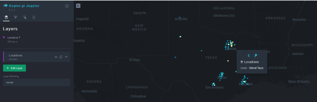

Then, we can display the results by simply calling location_map in the notebook. For convenience, we included the location_map_cfg Python dict in our notebook, which stores the settings necessary for the map to be created with the locations color-coded by chain. If we wish to make modifications to the map and save the new configuration for later use, we can do so by calling location_map.config and saving the result either as a cell in our notebook or in a separate location_map_cfg.py file.

Generating Isochrones

Now, for each of these locations, we can generate a polygon known as an isochrone or drivetime. These polygons will represent the areas that are within a certain time’s drive from the given location. We will generate these drivetimes using the Valhalla isochrone api:

def get_isochrone(lat, lng, costing, time_steps, name, location_id):
    url = "<https://valhalla1.openstreetmap.de/isochrone>"
    params = {
      "locations": [{"lon": lng, "lat": lat}],
      "contours": [{"time": i} for i in time_steps],
      "costing": costing,
      "polygons": 1,
    }
    response = requests.post(url, json=params)
    if response:
        result = response.json()
        if 'error_code' not in result.keys():
            df = gpd.GeoDataFrame.from_features(result)
            df['name'] = name
            df['id'] = location_id
            return df[['name','id','geometry']]

The function takes as its input a latitude and longitude value, a costing paratemeter, a location name, and a location id. The output is a dataframe which contains a Shapely polygon representing the isochrone, along with the a name and id of the location the isochrone corresponds to.

We have separate columns for a location id and a location name so that we can use the id column to examine isochrones for individual restaurants and we can use the name column to look at isochrones for each of the chains.

The costing parameter can take on several different values (see the API reference here), and it can be used to create “drivetimes” assuming the user is either walking, driving, or taking public transport.

We create a geoDataFrame of all of the 5-minute drivetimes for our taco restaurant locations

drivetimes_5_min = pd.concat([get_isochrone(row.lat, row.long, 'auto', [5],
 row.chain, row.id) for row in stores.select('id','chain','lat','long').collect()])

and then save it to our S3 storage for later use:

drivetimes_5_min.to_csv('s3://path/drivetimes_5_min_torchys_velvet.csv',
 index = False)

Because we are using a free API and we have to create quite a few of these isochrones, we highly recommend saving the file for later analysis. For the purposes of this blog, we have provided a ready-made isochrone file here, which we can load into Wherobots with the following snippet:

sedona.read.option('header','true').format('csv') .\\
load('s3://path/drivetimes_5_min_torchys_velvet.csv') .\\
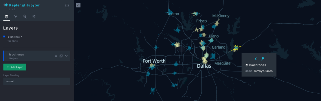
createOrReplaceTempView('drivetimes_5_min')

We can now visualize our drivetime polygons in SedonaKepler. As before, we first create the map with the snippet below.

map_isochrones = sedona.read.option('header','true').format('csv'). \\
load('s3://path/drivetimes_5_min_torchys_velvet.csv')

isochrone_map = SedonaKepler.create_map(map_isochrones, "Isochrones",
 config = isochrone_map_cfg)

Now, we can display the result by calling isochrone_map .

The Analysis

At this point, we have a collection of the Torchy’s and Velvet Taco locations in Texas, and we know the areas which are within a 5-minute drive of each location. What we want to do now is to estimate the number of potential customers that live near each of these locations, and the extent to which these populations overlap.

A First Look

Before we look at how these two chains might compete with each other, let’s also take a look at the extent to which restaurants within each chain might be cannibalizing each others’ sales. A quick way to do this is by using the filtering feature in Kepler to look at isochrones for a single chain:

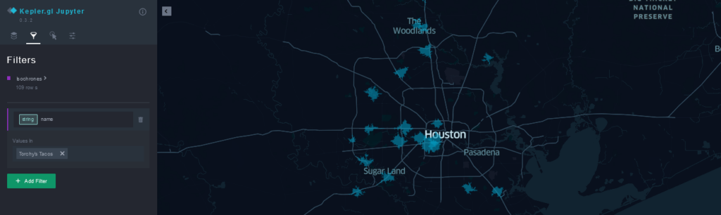
We see that locations for each chain are fairly spread out and (at least at the 5-minute drivetime level), there is not a high degree of cannibalization within each chain. Looking at the isochrones for both chains, however, we notice that Velvet Taco locations often tend to be near Torchy’s Tacos locations (or vice-versa). At this point, all we have are qualitative statements based on these maps. Next, we will show how to use H3 and existing open-source datasets to make these statements more quantitative.

Estimating Cannibalization Potential

As we can see by looking at the map of isochrones above, they are highly irregular polygons which have a considerable amount of overlap. In general, these polygons are not described in a ‘nice’ way by any administrative boundaries such as census block groups, census tracts, etc. Therefore, we will have to be a little creative in order to estimate the population inside them.

One way of doing this using the tools provided by Apache Sedona and Wherobots is to convert these polygons to H3 hexes. We can do this with the following snippet:

sedona.sql("""
SELECT ST_H3CellIds(ST_GeomFromWKT(geometry), 8, false) AS h3, name, id
FROM drivetimes_5_min
""").select(explode('h3'), 'name','id').withColumnRenamed('col','h3') .\\
createOrReplaceTempView('h3_isochrones')

This turns our table of drivetime polygons into a table where each row represents a hexagon with sides roughly 400m long, which is a part of a drivetime polygon. We also record the chain that these hexagons are associated to (the chain that the polygon they came from belongs to). We store each hexagon in its own row because this will simplify the process of estimating population later on.

Although the question of estimating population inside individual H3 hexes is also a difficult one (we will release a notebook on this soon), open-source datasets with this information are available online, and we will use one such dataset, provided by Kontur:

kontur = sedona.read.option('header','true') .\\
load('s3://path/us_h3_8_pop.geojson', format="json") .\\
drop('_corrupt_record').dropna() .\\
selectExpr('CAST(CONV(properties.h3, 16, 10) AS BIGINT) AS h3',
 'properties.population as population')

kontur.createOrReplaceTempView('kontur')

We can now enhance our h3_isochrones table with population counts for each H3 hex:

sedona.sql("""
SELECT ST_H3CellIds(ST_GeomFromWKT(geometry), 8, false) AS h3, name, id
FROM drivetimes_5_min
""").select(explode('h3'), 'name','id').withColumnRenamed('col','h3') .\\
join(kontur, 'h3', 'left').distinct().createOrReplaceTempView('h3_isochrones')

At this stage, we can also quickly compute the cannibalization potential within each chain. Using the following code, for example, we can estimate the number of people who live within a 5 minute drive of more than one Torcy’s Tacos:

sedona.sql("""
SELECT ST_H3CellIds(ST_GeomFromWKT(geometry), 8, false) AS h3, name, id
FROM drivetimes_5_min
""").select(explode('h3'), 'name','id').withColumnRenamed('col','h3') .\\
join(kontur, 'h3', 'left').filter('name LIKE "%Torchy%"').select('h3','population') .\\
groupBy('h3').count().filter('count >= 2').join(kontur, 'h3', 'left').distinct() .\\
agg(F.sum('population')).collect()[0][0]

97903.0

We can easily change this code to compute the same information for Velvet Taco by changing filter('name LIKE "%Torchy%"') in line 4 of the above snippet to filter('name LIKE "%Velvet%"') . If we do this, we will see that 100298 people live within a 5 minute drive of more than one Velvet Taco. Thus, we see that the Torchy’s Tacos brand appears to be slightly better at avoiding canibalization among its own locations (especially given that Torchy’s Tacos has more locations than Velvet Taco).

Now, we can run the following query to show the number of people in Texas who live within a 5 minutes drive of a Torchy’s Tacos:

sedona.sql("""
WITH distinct_h3 (h3, population) AS 
(
    SELECT DISTINCT h3, ANY_VALUE(population)
    FROM h3_isochrones
    WHERE name LIKE "%Torchy's%"
    GROUP BY h3
)
SELECT SUM(population)
FROM distinct_h3
""").show()

The reason we select distinct H3 hexes here is because a single hex can belong to more than one isochrone (as evidenced by the SedonaKepler visualizations above). We get the following output:

+---------------+
|sum(population)|
+---------------+
|      1546765.0|
+---------------+

So roughly 1.5 million people in Texas live within a 5-minute drive of a Torchy’s Tacos location. Looking at our previous calculations for how many people live near more than one restaurant of the same chain, we can see that Torchy’s Tacos locations near each other cannibalize about 6.3% of the potential customers who live within 5 minutes of a Torchy’s location.

Running a similar query for Velvet Taco tells us that roughly half as many people live within a 5-minute drive of a Velvet Taco:

sedona.sql("""
WITH distinct_h3 (h3, population) AS 
(
    SELECT DISTINCT h3, ANY_VALUE(population)
    FROM h3_isochrones
    WHERE name LIKE '%Velvet Taco%'
    GROUP BY h3
)
SELECT SUM(population)
FROM distinct_h3
""").show()

+---------------+
|sum(population)|
+---------------+
|       750360.0|
+---------------+

As before, we can also see that Velvet Taco locations near each other cannibalize about 13.4% of the potential customers who live within 5 minutes of a Velvet Taco location.

Now, we can estimate the potential for cannibalization between these two chains:

sedona.sql("""
WITH overlap_h3 (h3, population) AS
(
    SELECT DISTINCT a.h3, ANY_VALUE(a.population)
    FROM h3_isochrones a LEFT JOIN h3_isochrones b ON a.h3 = b.h3
    WHERE a.name != b.name
    GROUP BY a.h3
)
SELECT sum(population)
FROM overlap_h3
""").show()

which gives:

+---------------+
|sum(population)|
+---------------+
|       415033.0|
+---------------+

We can see that more than half of the people who live near a Velvet Taco location also live near a Torchy’s Tacos location and we can visualize this population overlap:

isochrones_h3_map_data = sedona.sql("""
SELECT ST_H3CellIds(ST_GeomFromWKT(geometry), 8, false) AS h3, name, id
FROM drivetimes_5_min
""").select(explode('h3'), 'name','id').withColumnRenamed('col','h3') .\
join(kontur, 'h3', 'left').select('name','population',array('h3')).withColumnRenamed('array(h3)','h3').selectExpr('name','population','ST_H3ToGeom(h3)[0] AS geometry')

isochrones_h3_map = SedonaKepler.create_map(isochrones_h3_map_data, 'Isochrones in H3', config = isochrones_h3_map_cfg)

Want to keep up with the latest developer news from the Wherobots and Apache Sedona community? Sign up for the This Month In Wherobots Newsletter: