Processing A Billion Aircraft Observations And Combining With Weather Data Using Apache Sedona On Wherobots Cloud
In this post we take a look at combining aircraft flight data with weather data to identify potentially impacted flights using public ADS-B data and weather data from NOAA. Along the way we introduce the types of spatial queries available with WherobotsDB including spatial range queries, spatial kNN, and spatial joins using Spatial SQL, geospatial […]
TABLE OF CONTENTS
Contributors
-
William Lyon
Developer Relations At Wherobots
In this post we take a look at combining aircraft flight data with weather data to identify potentially impacted flights using public ADS-B data and weather data from NOAA. Along the way we introduce the types of spatial queries available with WherobotsDB including spatial range queries, spatial kNN, and spatial joins using Spatial SQL, geospatial visualization options, working with various file formats including GeoParquet, GeoTiff, Shapefiles, and more.
We’ll be running this example in Wherobots Cloud, where you can create a free account to follow along. See the Getting Started With Wherobots Cloud series for an overview of Wherobots Cloud.
Flight Trace Data
The ADS-B flight observation data we’ll be using comes from ADSB.lol which provides publicly accessible daily updates of crowd-sourced flight tracking data. I adapted some great examples for downloading, parsing and enriching this dataset from Mark Litwintschik’s blog post and extracted 1 month of data which resulted in just over 1.1 billion observations. I extended Mark’s approach a bit and saved this data as GeoParquet, partitioned by S2 id. This will enable more efficient spatial queries on the dataset.
First, we’ll import dependencies and configure WherobotsDB to access an S3 bucket with our example data.
from sedona.spark import *

config = SedonaContext.builder().config("spark.hadoop.fs.s3a.bucket.wherobots-examples.aws.credentials.provider","org.apache.hadoop.fs.s3a.AnonymousAWSCredentialsProvider").getOrCreate()
sedona = SedonaContext.create(config)
We load one month of world-wide aircraft trace data which is just over 1.1 billion point observations.
# Load flight traces via GeoParquet
traces_df = sedona.read.format("geoparquet").load("s3a://wherobots-examples/data/examples/flights/2024_s2.parquet")
traces_df.createOrReplaceTempView("traces")

traces_df.count()
-------------------
1103371367
Exploratory Data Analysis
I followed Mark’s approach of extracting individual trace observations into their own row and we store detailed information about the trace such as altitude, squawk code, heading, etc in a struct. You can find his code in this post.
Let’s view the schema of our Spatial DataFrame that we loaded via GeoParquet.
traces_df.printSchema()root
|-- dbFlags: long (nullable = true)
|-- desc: string (nullable = true)
|-- icao: string (nullable = true)
|-- ownOp: string (nullable = true)
|-- r: string (nullable = true)
|-- reg_details: struct (nullable = true)
| |-- description: string (nullable = true)
| |-- iso2: string (nullable = true)
| |-- iso3: string (nullable = true)
| |-- nation: string (nullable = true)
|-- t: string (nullable = true)
|-- timestamp: string (nullable = true)
|-- trace: struct (nullable = true)
| |-- aircraft: struct (nullable = true)
| | |-- alert: long (nullable = true)
| | |-- alt_geom: long (nullable = true)
| | |-- baro_rate: long (nullable = true)
| | |-- category: string (nullable = true)
| | |-- emergency: string (nullable = true)
| | |-- flight: string (nullable = true)
| | |-- geom_rate: long (nullable = true)
| | |-- gva: long (nullable = true)
| | |-- ias: long (nullable = true)
| | |-- mach: double (nullable = true)
| | |-- mag_heading: double (nullable = true)
| | |-- nac_p: long (nullable = true)
| | |-- nac_v: long (nullable = true)
| | |-- nav_altitude_fms: long (nullable = true)
| | |-- nav_altitude_mcp: long (nullable = true)
| | |-- nav_heading: double (nullable = true)
| | |-- nav_modes: array (nullable = true)
| | | |-- element: string (containsNull = true)
| | |-- nav_qnh: double (nullable = true)
| | |-- nic: long (nullable = true)
| | |-- nic_baro: long (nullable = true)
| | |-- oat: long (nullable = true)
| | |-- rc: long (nullable = true)
| | |-- roll: double (nullable = true)
| | |-- sda: long (nullable = true)
| | |-- sil: long (nullable = true)
| | |-- sil_type: string (nullable = true)
| | |-- spi: long (nullable = true)
| | |-- squawk: string (nullable = true)
| | |-- tas: long (nullable = true)
| | |-- tat: long (nullable = true)
| | |-- track: double (nullable = true)
| | |-- track_rate: double (nullable = true)
| | |-- true_heading: double (nullable = true)
| | |-- type: string (nullable = true)
| | |-- version: long (nullable = true)
| | |-- wd: long (nullable = true)
| | |-- ws: long (nullable = true)
| |-- altitude: long (nullable = true)
| |-- flags: long (nullable = true)
| |-- geometric_altitude: long (nullable = true)
| |-- geometric_vertical_rate: long (nullable = true)
| |-- ground_speed: double (nullable = true)
| |-- h3_5: string (nullable = true)
| |-- indicated_airspeed: long (nullable = true)
| |-- lat: double (nullable = true)
| |-- lon: double (nullable = true)
| |-- roll_angle: double (nullable = true)
| |-- source: string (nullable = true)
| |-- timestamp: string (nullable = true)
| |-- track_degrees: double (nullable = true)
| |-- vertical_rate: long (nullable = true)
|-- year: string (nullable = true)
|-- geometry: geometry (nullable = true)
|-- date: date (nullable = true)
|-- s2: long (nullable = true)
We can also inspect the first few rows of data.
traces_df.show(5)+-------+--------------------+------+-----+------+--------------------+----+-------------------+--------------------+----+--------------------+----------+-------------------+
|dbFlags| desc| icao|ownOp| r| reg_details| t| timestamp| trace|year| geometry| date| s2|
+-------+--------------------+------+-----+------+--------------------+----+-------------------+--------------------+----+--------------------+----------+-------------------+
| 0|PIPER PA-28R-180/...|c81c51| null|ZK-RTE|{general, NZ, NZL...|P28R|2024-01-20 00:00:00|{{null, null, nul...|null|POINT (174.722786...|2024-01-20|7854277750134145024|
| 0| AIRBUS A-320|c81e2c| null|ZK-OJS|{general, NZ, NZL...|A320|2024-01-15 00:00:00|{{0, 36400, 0, A3...|null|POINT (174.549826...|2024-01-15|7854277750134145024|
| 0|PIPER PA-28R-180/...|c81c51| null|ZK-RTE|{general, NZ, NZL...|P28R|2024-01-20 00:00:00|{{null, null, nul...|null|POINT (174.722764...|2024-01-20|7854277750134145024|
| 0| AIRBUS A-320|c81e2c| null|ZK-OJS|{general, NZ, NZL...|A320|2024-01-15 00:00:00|{{null, null, nul...|null|POINT (174.557251...|2024-01-15|7854277750134145024|
| 0|PIPER PA-28R-180/...|c81c51| null|ZK-RTE|{general, NZ, NZL...|P28R|2024-01-20 00:00:00|{{0, 1600, null, ...|null|POINT (174.722589...|2024-01-20|7854277750134145024|
+-------+--------------------+------+-----+------+--------------------+----+-------------------+--------------------+----+--------------------+----------+-------------------+
only showing top 5 rows
We can query our aircraft traces Spatial DataFrame using Spatial SQL. To start off let’s just demonstrate selecting fields and viewing tabular results. Note that the geometry column here is a spatial type. The data we loaded was GeoParquet formatted so we don’t need to parse or cast the field to a geometry type.
sedona.sql("""
SELECT desc, ownOp, geometry, trace.ground_speed, trace.altitude, trace.aircraft.flight
FROM traces
WHERE trace.altitude IS NOT NULL AND OwnOp IS NOT NULL AND desc IS NOT NULL AND trace.aircraft.flight IS NOT NULL
LIMIT 10
""").show(truncate=False)
+----------------+-------------------+-----------------------------+------------+--------+--------+
|desc |ownOp |geometry |ground_speed|altitude|flight |
+----------------+-------------------+-----------------------------+------------+--------+--------+
|AIRBUS A-350-900|UMB BANK NA TRUSTEE|POINT (174.792839 -37.010239)|122.7 |400 |DAL64 |
|AIRBUS A-350-900|UMB BANK NA TRUSTEE|POINT (174.782449 -37.013079)|161.6 |350 |DAL64 |
|AIRBUS A-350-900|UMB BANK NA TRUSTEE|POINT (174.779046 -37.01401) |168.9 |475 |DAL64 |
|AIRBUS A-350-900|UMB BANK NA TRUSTEE|POINT (174.771463 -37.016058)|165.7 |825 |DAL64 |
|AIRBUS A-350-900|UMB BANK NA TRUSTEE|POINT (174.765248 -37.017746)|162.5 |1175 |DAL64 |
|AIRBUS A-350-900|UMB BANK NA TRUSTEE|POINT (174.757827 -37.01976) |159.4 |1550 |DAL64 |
|AIRBUS A-350-900|UMB BANK NA TRUSTEE|POINT (174.748356 -37.022296)|161.3 |1950 |DAL64 |
|AIRBUS A-350-900|UMB BANK NA TRUSTEE|POINT (174.738951 -37.024796)|163.2 |2325 |DAL64 |
|AIRBUS A-350-900|UMB BANK NA TRUSTEE|POINT (174.725607 -37.028395)|165.7 |2725 |DAL64 |
|AIRBUS A-350-900|UMB BANK NA TRUSTEE|POINT (174.713367 -37.03184) |167.3 |3125 |DAL64 |
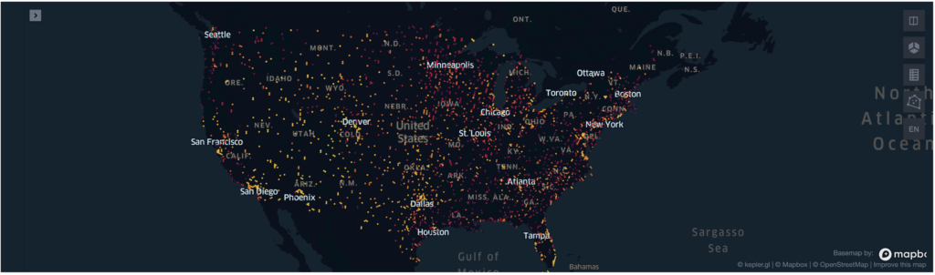
+----------------+-------------------+-----------------------------+------------+--------+--------+Let’s see where the aircraft activity is in the ADS-B flight observation dataset. Where are we seeing the most aircraft activity? We can use H3 hexagons to aggregate the individual traces and visualize the results using the SedonaKepler visualization integration. Here we count the number of aircraft trace observations within each level 5 H3 hexagon and create a choropleth map to visualize the spatial distribution.
h3_traces_df = sedona.sql("""
SELECT
    COUNT(*) AS num,
    ST_H3ToGeom(ST_H3CellIDs(geometry, 5, false)) AS geometry,
    ST_H3CellIDs(geometry, 5, false) AS h3
FROM traces
GROUP BY h3
""")

SedonaKepler.create_map(h3_traces_df, name="Distribution of aircraft traces")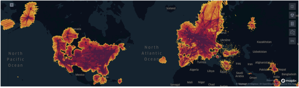
Since our data source relies on crowdsourced data retrieved from ground stations, the data coverage is not evenly distributed. We are notably missing observations over the oceans and other areas that lack crowd-sourced ground sensors. This isn’t an issue for this analysis because flight disruption is most likely to occur around airports.
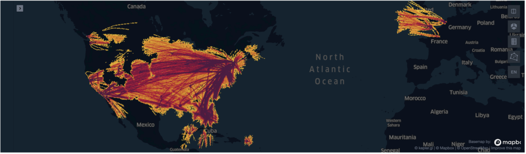
We can filter for aircraft belonging to a specific airline using the ownOp column and also filter for traces that were observed while the aircraft was part of a named flight. This can help give us some insight into the routes flown by this airline.
jbu_h3_traces_df = sedona.sql("""
SELECT
    COUNT(*) AS num,
    ST_H3ToGeom(ST_H3CellIDs(geometry, 5, false)) AS geometry,
    ST_H3CellIDs(geometry, 5, false) AS h3
FROM traces
WHERE ownOp = "JETBLUE AIRWAYS CORP" AND trace.aircraft.flight LIKE "JBU%"
GROUP BY h3
""")

SedonaKepler.create_map(jbu_h3_traces_df, name="Distribution of aircraft traces")
Flight Traces – Spatial Queries And Performance
WherobotsDB supports optimizations for various types of spatial queries including:
- Spatial range query
- Spatial kNN query, and
- Spatial joins
Let’s demonstrate these types of queries and compare the performance with this dataset.
Spatial Range Query
Let’s say we wanted to find all aircraft traces within the bounds of a specific area, perhaps the Gulf of Mexico region. We can do this using the ST_Within Spatial SQL predicate.
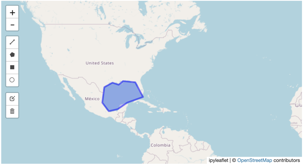
Here we apply this spatial predicate to filter our 1.1 billion observations to only those within the bounds of a polygon representing a specific area. This takes just over 4 seconds.
gulf_filter = 'ST_Within(geometry, ST_GeomFromWKT("POLYGON ((-84.294662 29.840644, -88.952866 30.297018, -89.831772 28.767659, -94.050522 29.61167, -97.038803 27.839076, -97.917709 21.453069, -94.489975 18.479609, -86.843491 21.616579, -80.779037 24.926295, -84.294662 29.840644))"))'
gulf_traces = traces_df.where(gulf_filter)

%%time
gulf_traces.count()
--------------------
7539347

Wall time: 4.37 s
Spatial kNN Query
Another type of spatial query that might be relevant for working with this dataset is a spatial kNN query, which will efficiently find the “k” nearest geometries where the value of k is specified by the user. For example, let’s find the 5 nearest aircraft traces to the Jackson Hole Airport.
jackson_hole_traces = sedona.sql("""
SELECT
    desc,
    ownOp,
    trace.aircraft.flight,
    ST_DistanceSphere(ST_Point(-110.7376, 43.6088), geometry) AS distance
FROM traces
ORDER BY distance ASC
LIMIT 5
""")

%%time

jackson_hole_traces.show()
----------------------------
Wall time: 11.1 s
+--------------------+--------------------+--------+------------------+
| desc| ownOp| flight| distance|
+--------------------+--------------------+--------+------------------+
|BOMBARDIER BD-700...| FLEXJET LLC| null| 76.92424103100763|
| AIRBUS A-320| UNITED AIRLINES INC| null|161.98830220247405|
|CESSNA 700 CITATI...|AH CAPITAL MANAGE...| null|180.05761405860687|
|CESSNA 750 CITATI...| 2FLIU LLC| null|187.01797656145476|
|DASSAULT FALCON 2000|NEXTERA ENERGY EQ...|N58MW |204.06240031528034|
+--------------------+--------------------+--------+------------------+In this case our query takes 11 seconds against a 1.1 billion row dataset.
Historical Impact of Severe Weather Events On Flights
An important analysis related to flight routes is the impact of severe weather events. To enable this type of analysis Wherobots makes public a dataset of severe weather events as part of the Wherobots Open Data Catalog. The dataset has over 8 million weather events reported by NOAA in the US from 2016-2022.
weather = sedona.table("wherobots_pro_data.weather.weather_events")
weather.show()
+--------+-------------+--------+-------------------+-------------------+-----------------+----------+-----------+-----------+-----------+----+--------------+-----+-------+--------------------+
| EventId| Type|Severity| StartTime(UTC)| EndTime(UTC)|Precipitation(in)| TimeZone|AirportCode|LocationLat|LocationLng|City| County|State|ZipCode| geometry|
+--------+-------------+--------+-------------------+-------------------+-----------------+----------+-----------+-----------+-----------+----+--------------+-----+-------+--------------------+
|W-237263| Cold| Severe|2016-01-01 08:57:00|2016-01-04 15:32:00| 0.0|US/Pacific| KNSI| 33.2338| -119.4559|null|Ventura County| CA| null|POINT (-119.4559 ...|
|W-237264| Rain| Light|2016-01-04 22:49:00|2016-01-04 23:30:00| 0.0|US/Pacific| KNSI| 33.2338| -119.4559|null|Ventura County| CA| null|POINT (-119.4559 ...|
|W-237265| Cold| Severe|2016-01-05 00:35:00|2016-01-05 15:32:00| 0.0|US/Pacific| KNSI| 33.2338| -119.4559|null|Ventura County| CA| null|POINT (-119.4559 ...|
|W-237266| Rain| Light|2016-01-05 15:32:00|2016-01-05 17:57:00| 0.2|US/Pacific| KNSI| 33.2338| -119.4559|null|Ventura County| CA| null|POINT (-119.4559 ...|
|W-237267| Rain|Moderate|2016-01-05 17:57:00|2016-01-05 18:09:00| 0.14|US/Pacific| KNSI| 33.2338| -119.4559|null|Ventura County| CA| null|POINT (-119.4559 ...|
|W-237268| Rain| Light|2016-01-05 18:09:00|2016-01-05 18:23:00| 0.07|US/Pacific| KNSI| 33.2338| -119.4559|null|Ventura County| CA| null|POINT (-119.4559 ...|
|W-237269| Rain|Moderate|2016-01-05 18:23:00|2016-01-05 18:57:00| 0.35|US/Pacific| KNSI| 33.2338| -119.4559|null|Ventura County| CA| null|POINT (-119.4559 ...|
|W-237270|Precipitation| UNK|2016-01-05 18:57:00|2016-01-05 19:41:00| 0.22|US/Pacific| KNSI| 33.2338| -119.4559|null|Ventura County| CA| null|POINT (-119.4559 ...|
|W-237271| Cold| Severe|2016-01-06 00:57:00|2016-01-06 15:31:00| 0.0|US/Pacific| KNSI| 33.2338| -119.4559|null|Ventura County| CA| null|POINT (-119.4559 ...|
|W-237272| Rain| Light|2016-01-06 16:57:00|2016-01-06 18:33:00| 0.16|US/Pacific| KNSI| 33.2338| -119.4559|null|Ventura County| CA| null|POINT (-119.4559 ...|
|W-237273|Precipitation| UNK|2016-01-06 18:57:00|2016-01-06 19:10:00| 0.23|US/Pacific| KNSI| 33.2338| -119.4559|null|Ventura County| CA| null|POINT (-119.4559 ...|
|W-237274| Rain|Moderate|2016-01-06 19:10:00|2016-01-06 19:57:00| 0.16|US/Pacific| KNSI| 33.2338| -119.4559|null|Ventura County| CA| null|POINT (-119.4559 ...|
|W-237275| Rain| Light|2016-01-06 20:57:00|2016-01-06 21:27:00| 0.03|US/Pacific| KNSI| 33.2338| -119.4559|null|Ventura County| CA| null|POINT (-119.4559 ...|
|W-237276| Rain|Moderate|2016-01-06 21:27:00|2016-01-06 22:57:00| 0.26|US/Pacific| KNSI| 33.2338| -119.4559|null|Ventura County| CA| null|POINT (-119.4559 ...|
|W-237277| Cold| Severe|2016-01-07 00:57:00|2016-01-07 15:35:00| 0.0|US/Pacific| KNSI| 33.2338| -119.4559|null|Ventura County| CA| null|POINT (-119.4559 ...|
|W-237278| Rain| Light|2016-01-07 18:10:00|2016-01-07 18:57:00| 0.0|US/Pacific| KNSI| 33.2338| -119.4559|null|Ventura County| CA| null|POINT (-119.4559 ...|
|W-237279| Rain| Light|2016-01-07 23:57:00|2016-01-08 00:57:00| 0.0|US/Pacific| KNSI| 33.2338| -119.4559|null|Ventura County| CA| null|POINT (-119.4559 ...|
|W-237280| Cold| Severe|2016-01-08 00:57:00|2016-01-08 15:29:00| 0.0|US/Pacific| KNSI| 33.2338| -119.4559|null|Ventura County| CA| null|POINT (-119.4559 ...|
|W-237281| Cold| Severe|2016-01-09 00:57:00|2016-01-11 14:32:00| 0.0|US/Pacific| KNSI| 33.2338| -119.4559|null|Ventura County| CA| null|POINT (-119.4559 ...|
|W-237282| Cold| Severe|2016-01-12 00:57:00|2016-01-12 15:57:00| 0.0|US/Pacific| KNSI| 33.2338| -119.4559|null|Ventura County| CA| null|POINT (-119.4559 ...|
+--------+-------------+--------+-------------------+-------------------+-----------------+----------+-----------+-----------+-----------+----+--------------+-----+-------+--------------------+
only showing top 20 rowsSevere Weather Events
Let’s start our weather event analysis by finding areas that are commonly susceptible to severe weather events. We’ll again use H3 hexagons to aggregate the data, this time counting the number of severe weather events that occur within each hexagon. We’ll visualize the results as a choropleth to see areas where weather events frequently occur.
weather_h3_df = sedona.sql("""
SELECT
    COUNT(*) AS num,
    ST_H3ToGeom(ST_H3CellIDs(ST_Buffer(geometry, 0.1), 5, false)) AS geometry,
    ST_H3CellIDs(ST_Buffer(geometry, 0.1), 5, false) AS h3
FROM wherobots_pro_data.weather.weather_events
WHERE Severity = "Severe"
GROUP BY h3
""")

weather_h3_df.createOrReplaceTempView("weather_h3")
SedonaKepler.create_map(weather_h3_df.cache(), name="Severe weather events")
Historical Severe Weather Aircraft Trace Analysis
Now that we’ve determined which areas are susceptible to frequent severe weather events, we can analyze flight trace observations in these areas to determine flights that may be susceptible to frequent severe weather events using a spatial join. Note that we’re joining a table with 1.1 billion observations against our weather event data, which takes just under 13 seconds in Wherobots Cloud.
severe_weather_flight_traces_df= sedona.sql("""
SELECT traces.geometry AS geometry, desc, ownOp, trace.aircraft.flight AS flight, num AS eventCount
FROM traces
JOIN weather_h3
WHERE ST_Contains(weather_h3.geometry, traces.geometry) AND trace.aircraft.flight IS NOT null
""")

%%time
severe_weather_flight_traces_df.count()
----------------------------
Wall time: 12.7 s

53788395
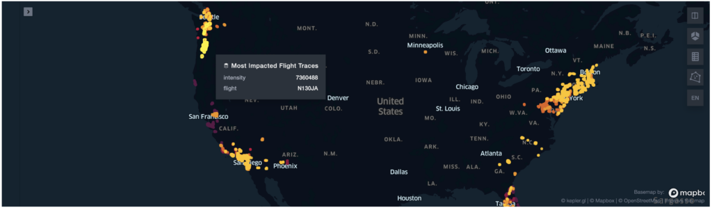
Using the flight number we can calculate an “intensity” metric that attempts to measure the potential impact of a flight to be disrupted by a severe weather event using the historical weather data. Here we calculate this intensity metric across all traces to find the most potentially impacted flights.
most_impacted_flights = sedona.sql("""
SELECT sum(eventCount) AS intensity, ST_Collect(collect_list(geometry)) AS geometry, flight
FROM severe_weather_traces
WHERE NOT flight = "        " AND NOT flight = "00000000"
GROUP BY flight
ORDER BY intensity DESC
LIMIT 100
""")
Flight Routes
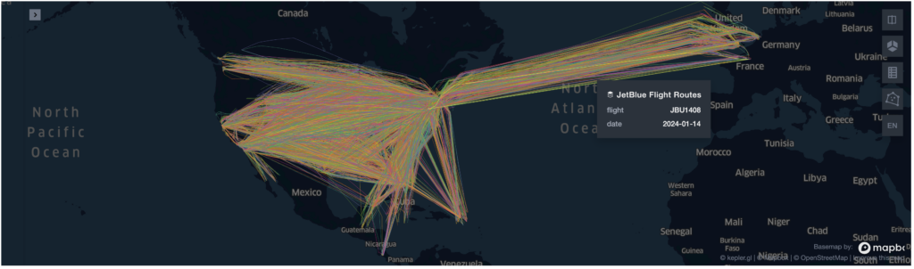
So far we’ve been working with individual aircraft traces (point observations), but it’s much more useful to analyze flights as routes. We can construct the individual flight routes from these aircraft traces, for a specific airline by filtering on the ownOp and trace.aircraft.flight fields.
First we collect all aircraft traces that match our filter by airline, grouping by flight number. Then we can convert this collection of point geometries into a LineString geometry that represents the path the aircraft took during this flight using the ST_MakeLine Spatial SQL function.
jbu_flights_df = sedona.sql("""
WITH jbu_traces AS (
    SELECT
        any_value(trace.aircraft.flight) AS flight,
        collect_list(ST_Point(trace.lon, trace.lat)) AS points,
        any_value(CAST(date AS string)) AS date
    FROM traces
    WHERE ownOp = 'JETBLUE AIRWAYS CORP' AND trace.aircraft.flight IS NOT null
    GROUP BY trace.aircraft.flight, date
)
SELECT flight, ST_MakeLine(points) AS geometry, date
FROM jbu_traces
WHERE size(points) > 100
""")

jbu_flights_df.show()
+--------+--------------------+----------+
|  flight|            geometry|      date|
+--------+--------------------+----------+
|JBU100  |LINESTRING (-112....|2024-01-24|
|JBU101  |LINESTRING (-80.1...|2024-01-21|
|JBU1016 |LINESTRING (-77.3...|2024-01-20|
|JBU1044 |LINESTRING (-80.1...|2024-01-10|
|JBU1053 |LINESTRING (-73.7...|2024-01-03|
|JBU1055 |LINESTRING (-71.0...|2024-01-03|
|JBU1060 |LINESTRING (-77.4...|2024-01-12|
|JBU1060 |LINESTRING (-77.4...|2024-01-26|
|JBU1067 |LINESTRING (-73.7...|2024-01-17|
|JBU1068 |LINESTRING (-80.0...|2024-01-24|
|JBU1114 |LINESTRING (-112....|2024-01-17|
|JBU1131 |LINESTRING (-80.2...|2024-01-22|
|JBU1136 |LINESTRING (-83.3...|2024-01-15|
|JBU1142 |LINESTRING (-80.0...|2024-01-27|
|JBU1196 |LINESTRING (-80.1...|2024-01-03|
|JBU1196 |LINESTRING (-80.1...|2024-01-27|
|JBU1217 |LINESTRING (-81.6...|2024-01-15|
|JBU1230 |LINESTRING (-86.8...|2024-01-22|
|JBU1238 |LINESTRING (-97.6...|2024-01-28|
|JBU1251 |LINESTRING (-73.7...|2024-01-10|
+--------+--------------------+----------+
only showing top 20 rows
Identify Potential For Weather Impacted Flights
Now that we’ve extracted flight routes from the individual aircraft trace point observations we can begin to determine the potential for severe weather events to impact these flights based on our historical weather event data.
Creating Uniform Flight Route Segments
To analyze which flights have the most potential to be impacted based on historical weather events we first create 100km segments of each flight which will allow us to identify not only entire flight routes that are potentially impacted by weather events, but specific flight segments with the most risk of disruption.
To do this we’ll make use of the ability to create a user defined function in WherobotsDB using the Shapely library. We’ll use Shapely’s line interpolate functionality to create equal length segments of each flight route.
from shapely.geometry import LineString, MultiLineString
from sedona.sql.types import GeometryType

# Define a Shapely UDF to create a series of consistent length line segments for each flight
def interpolate_lines(line: GeometryType()):
    try:
        distance_delta = 1.0 # ~100km
        points_count = int(line.length // distance_delta) + 1
        distances = (distance_delta * i for i in range(points_count))
        points = [line.interpolate(distance) for distance in distances] + [line.boundary[1]]
        line_strings = []
        for i in range(len(points) - 1):
            line_strings.append(LineString([points[i], points[i+1]]))
        return MultiLineString(line_strings)
    except:
        return None

sedona.udf.register("interpolate_lines", interpolate_lines, GeometryType())
We can now call our user defined function in a spatial SQL statement and leverage WherobotsDB’s parallel execution to run this UDF.
split_df = sedona.sql("""
SELECT flight, date, explode(ST_Dump(interpolate_lines(geometry))) AS geometry
FROM jbu_flights
""")

split_df.createOrReplaceTempView("split_flights")
split_df.show()
+--------+----------+--------------------+
|  flight|      date|            geometry|
+--------+----------+--------------------+
|JBU100  |2024-01-24|LINESTRING (-118....|
|JBU100  |2024-01-24|LINESTRING (-117....|
|JBU100  |2024-01-24|LINESTRING (-116....|
|JBU100  |2024-01-24|LINESTRING (-115....|
|JBU100  |2024-01-24|LINESTRING (-114....|
|JBU100  |2024-01-24|LINESTRING (-113....|
|JBU100  |2024-01-24|LINESTRING (-112....|
|JBU100  |2024-01-24|LINESTRING (-111....|
|JBU100  |2024-01-24|LINESTRING (-110....|
|JBU100  |2024-01-24|LINESTRING (-109....|
|JBU100  |2024-01-24|LINESTRING (-108....|
|JBU100  |2024-01-24|LINESTRING (-107....|
|JBU100  |2024-01-24|LINESTRING (-106....|
|JBU100  |2024-01-24|LINESTRING (-105....|
|JBU100  |2024-01-24|LINESTRING (-104....|
|JBU100  |2024-01-24|LINESTRING (-103....|
|JBU100  |2024-01-24|LINESTRING (-102....|
|JBU100  |2024-01-24|LINESTRING (-102....|
|JBU100  |2024-01-24|LINESTRING (-101....|
|JBU100  |2024-01-24|LINESTRING (-100....|
+--------+----------+--------------------+
only showing top 20 rows
Joining Flight Route Segments With Weather Events
Now we perform a spatial join to identify flight segments that pass through areas that historically have a high frequency of severe weather events.
severe_weather_split_df = sedona.sql("""
SELECT flight, date, split_flights.geometry AS geometry, num
FROM split_flights
JOIN weather_h3
WHERE ST_Intersects(weather_h3.geometry, split_flights.geometry)
""")

severe_weather_split_df.show()
This gives us a measure of which individual flight segments have the highest potential for weather impact.
+--------+----------+--------------------+----+
|  flight|      date|            geometry| num|
+--------+----------+--------------------+----+
|JBU2288 |2024-01-02|LINESTRING (-69.3...|1221|
|JBU2288 |2024-01-02|LINESTRING (-70.3...|1774|
|JBU2288 |2024-01-02|LINESTRING (-71.2...|  42|
|JBU2288 |2024-01-02|LINESTRING (-71.2...|1192|
|JBU2288 |2024-01-02|LINESTRING (-71.2...|1231|
|JBU2288 |2024-01-02|LINESTRING (-72.2...| 672|
|JBU2288 |2024-01-02|LINESTRING (-72.2...| 959|
|JBU2288 |2024-01-02|LINESTRING (-73.2...| 652|
|JBU2288 |2024-01-02|LINESTRING (-73.2...| 672|
|JBU1053 |2024-01-03|LINESTRING (-73.7...| 416|
|JBU2424 |2024-01-07|LINESTRING (-81.2...| 217|
|JBU2424 |2024-01-07|LINESTRING (-81.2...| 467|
|JBU2424 |2024-01-07|LINESTRING (-81.2...| 487|
|JBU2424 |2024-01-07|LINESTRING (-81.2...| 611|
|JBU2424 |2024-01-07|LINESTRING (-81.3...| 885|
|JBU2424 |2024-01-07|LINESTRING (-81.3...| 722|
|JBU2424 |2024-01-07|LINESTRING (-81.3...|2237|
|JBU2424 |2024-01-07|LINESTRING (-81.3...| 722|
|JBU2424 |2024-01-07|LINESTRING (-81.3...| 618|
|JBU2424 |2024-01-07|LINESTRING (-81.3...| 607|
+--------+----------+--------------------+----+
only showing top 20 rows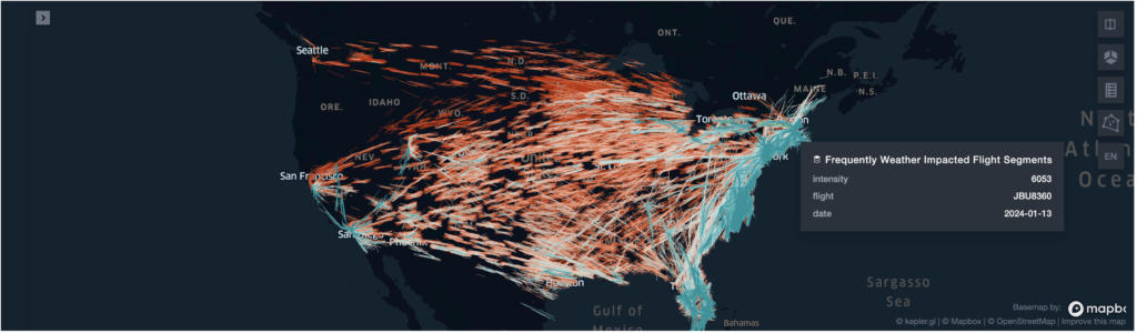
Flights With The Highest Potential For Weather Impact
Now we can join the flight segments and their corresponding weather intensity impact scores with the full flight routes to visualize the flights with the highest potential for weather impact based on the historical weather events.
full_flight_intensity_df = sedona.sql("""
SELECT jbu_flights.flight, jbu_flights.geometry, jbu_flights.date, intensity
FROM jbu_flights
JOIN jbu_intensity ON jbu_flights.flight = jbu_intensity.flight AND jbu_flights.date = jbu_intensity.date
""")

map_view = SedonaKepler.create_map(full_flight_intensity_df.orderBy("intensity", ascending=False).limit(10), name="Flights")
SedonaKepler.add_df(map_view, df=weather_h3_df, name="Weather")
map_view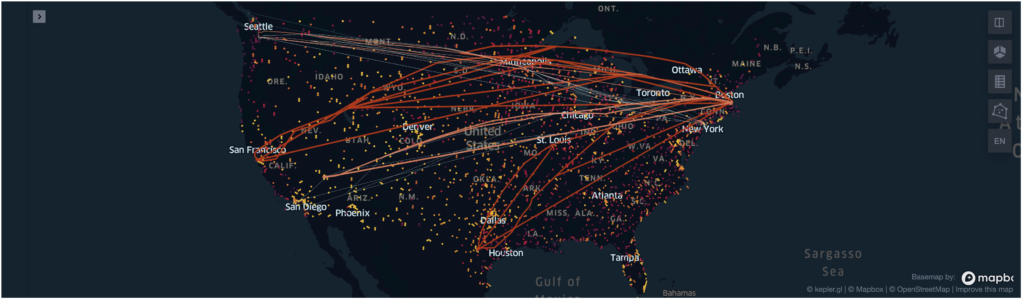
Doppler Weather Raster Data
So far we’ve been working with historical weather event data, lets now look at a simple example using more real-time weather radar data. Specifically, we’ll use NOAA’s NEXRAD Doppler weather radar surface reflectivity product to assess the impact of high precipitation at airports.
We’ll load a GeoTiff raster image of the continental US to identify weather patterns, then join this raster data with the location of US airports.
First, we load the raster image from S3 using the RS_FromPath function which will create an out-db raster in WherobotsDB.
nexrad_raster_url = "s3://wherobots-examples/data/noaa/nexrad/n0q_202309231625.tif"
nexrad_df = sedona.sql(f"SELECT RS_FromPath('{nexrad_raster_url}') AS raster")
nexrad_df.createOrReplaceTempView("nexrad")
nexrad_df.printSchema()
root
|-- raster: raster (nullable = true)Inspecting the meta data for this raster image we can see the spatial extent, spatial resolution, the CRS, and number of bands.
sedona.sql("SELECT RS_MetaData(raster) from nexrad").show(truncate=False)
+---------------------------------------------------------------------------+
|rs_metadata(raster)                                                        |
+---------------------------------------------------------------------------+
|[-126.0025, 50.0025, 12200.0, 5400.0, 0.005, -0.005, 0.0, 0.0, 4326.0, 1.0]|
+---------------------------------------------------------------------------+
We can visualize the raster using RS_AsImage.
htmlDf = sedona.sql("SELECT RS_AsImage(raster, 1200) AS raster_image FROM nexrad")
SedonaUtils.display_image(htmlDf)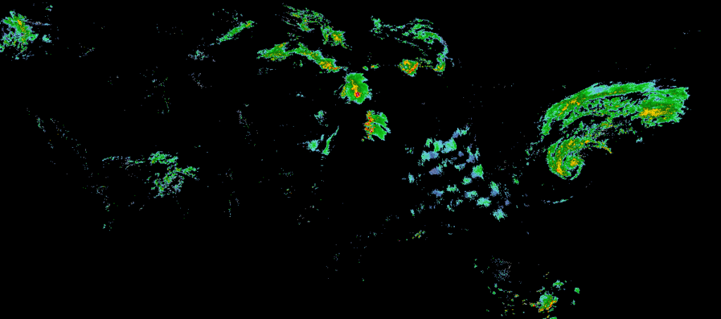
Next, we’ll load the point geometries of airports from a Shapefile.
spatialRdd = ShapefileReader.readToGeometryRDD(sedona.sparkContext, "s3a://wherobots-examples/data/ne_50m_airports")
poi_df = Adapter.toDf(spatialRdd, sedona)

poi_df = poi_df
poi_df.show(5)
poi_df.createOrReplaceTempView("airports")
+--------------------+---------+----------+-----+----------------+------+--------+--------+---------+--------------------+---------+
| geometry|scalerank|featurecla| type| name|abbrev|location|gps_code|iata_code| wikipedia|natlscale|
+--------------------+---------+----------+-----+----------------+------+--------+--------+---------+--------------------+---------+
|POINT (113.935016...| 2| Airport|major| Hong Kong Int'l| HKG|terminal| VHHH| HKG|http://en.wikiped...| 150.000|
|POINT (121.231370...| 2| Airport|major| Taoyuan| TPE|terminal| RCTP| TPE|http://en.wikiped...| 150.000|
|POINT (4.76437693...| 2| Airport|major| Schiphol| AMS|terminal| EHAM| AMS|http://en.wikiped...| 150.000|
|POINT (103.986413...| 2| Airport|major|Singapore Changi| SIN|terminal| WSSS| SIN|http://en.wikiped...| 150.000|
|POINT (-0.4531566...| 2| Airport|major| London Heathrow| LHR| parking| EGLL| LHR|http://en.wikiped...| 150.000|
+--------------------+---------+----------+-----+----------------+------+--------+--------+---------+--------------------+---------+
only showing top 5 rows
And now we’re ready to join the raster radar data to our vector airport locations. This operation retrieves the pixel value (in this case a precipitation index value) from the raster at the location of each airport. We’ll filter for any airports where this index value is above 100, indicating significant precipitation.
airport_precip_df = sedona.sql("""
SELECT name, iata_code, type, RS_Value(raster, geometry, 1) AS precip
FROM airports
JOIN nexrad
""")

airport_precip_df.where("precip > 100").show(truncate=False)
+-------------------+---------+-----+------+
|name               |iata_code|type |precip|
+-------------------+---------+-----+------+
|Gen E L Logan Int'l|BOS      |major|108.0 |
|Durham Int'l       |RDU      |major|138.0 |
+-------------------+---------+-----+------+
Based on this analysis we can see that Logan International Airport and Raleigh-Durham Airport are experiencing high precipitation events, which may potentially impact ground operations.
Resources
This blog post looked at combining aircraft trace observations from public ADS-B sensors with weather event and radar data to analyze the potential impact of severe weather events on flights.
You can follow along with these examples by creating a free account on Wherobots Cloud and find the code for this example on GitHub.
Learn more about this use case and Wherobots Cloud in a live demo Flight Analysis With Wherobots Cloud on June 20th at 8am Pacific time.
Contributors
-
William Lyon
Developer Relations At Wherobots