Hello Apache Sedona community,

We’re exhilarated to share the launch of Apache Sedona 1.4 (https://sedona.apache.org/1.4.1/), encompassing both 1.4.0 and 1.4.1 versions, signifying a transformative stage in geospatial analytics. These successive versions introduce an array of striking new features, major enhancements, and indispensable bug fixes.

Top-Notch Highlights

Here are the standout features spanning across these two versions:

1. Use SedonaContext as a unified entry point (SEDONA-287): This allows you to use the same method to initialize your Sedona environment in different computation engines without tedious configuration.
2. Geodesic/Geography Functions Support (SEDONA-281, SEDONA-286): This functionality adds a whole new dimension to your geospatial data processing, enabling more accurate computations over geographical data.
3. Redesigned end-to-end raster ETL pipeline (SEDONA-251, SEDONA-269, SEDONA-292): Apache Sedona 1.4 includes new raster readers / writers, raster type, and many essential raster functions, paving the way for streamlined handling of vast volumes of geospatial data.
4. Google S2 based spatial join (SEDONA-235): Sedona 1.4 introduces the support of Google S2 cells which enables a speedy approximate point-in-polygon join.
5. Support for Spark 3.4 (SEDONA-276): Our support for Spark 3.4 allows you to merge the powerful capabilities of the latest Spark version with the enhanced geospatial features of Sedona.
6. Serialization and Deserialization Enhancements (SEDONA-207, SEDONA-227, SEDONA-231): Sedona 1.4 offered faster geometry serialization and deserialization, resulting in a performance boost by a factor of 3 to 7.
7. Native filter pushdown support in GeoParquet (SEDONA-156): this can push down spatial predicate on GeoParquet to reduce memory consumption by 10X.

Now, let’s dive into Features 1-4 and learn how to leverage them in your applications. We’ll discuss the remaining features in separate blog posts.

Use SedonaContext as a unified entry point (v1.4.1)

Initially designed to be a geospatial computation system on top of Apache Spark, Sedona has evolved over the years. It has extended its support to other engines and is now on a mission to become a cross-platform, scalable geospatial computation engine.

To use Sedona with different underlying engines, you must import several classes and register necessary Sedona data types, serializers, functions, and optimization rules. This process can be confusing for new users over time. Let’s examine the Sedona Spark Python interface as an example:

Old Sedona entry point

from sedona.register import SedonaRegistrator
from sedona.core.SpatialRDD import SpatialRDD
from sedona.utils.adapter import Adapter
from sedona.core.spatialOperator import JoinQueryRaw
from sedona.core.formatMapper.shapefileParser import ShapefileReader
from sedona.sql.types import GeometryType
from sedona.core.enums import GridType
from sedona.core.enums import IndexType
from sedona.utils import SedonaKryoRegistrator, KryoSerializer

spark = SparkSession.\
    builder.\
    master("local[*]").\
    appName("Sedona App").\
    config("spark.serializer", KryoSerializer.getName).\
    config("spark.kryo.registrator", SedonaKryoRegistrator.getName) .\
    config("spark.jars.packages", "org.apache.sedona:sedona-spark-shaded-3.0_2.12:1.4.0,org.datasyslab:geotools-wrapper:1.4.0-28.2") .\
    getOrCreate()

SedonaRegistrator.registerAll(spark)

spatialDf = sedona.sql("SELECT ST_GeomFromWKT(XXX) FROM")

Users previously had to manually import many classes and add serializer configuration.

However, with the introduction of SedonaContext and other helper functions in SEDONA-287, starting applications has become much easier. Here’s how to do it:

SedonaContext with Spark Python

from sedona.spark import *

config = SedonaContext.builder() .\
    config('spark.jars.packages',
           'org.apache.sedona:sedona-spark-shaded-3.0_2.12:1.4.1,'
           'org.datasyslab:geotools-wrapper:1.4.0-28.2'). \
    getOrCreate()

sedona = SedonaContext.create(config)

spatialDf = sedona.sql("SELECT ST_GeomFromWKT(XXX) FROM")

SedonaContext with Flink Java

import org.apache.sedona.flink.SedonaContext

StreamTableEnvironment sedona = SedonaContext.create(env, tableEnv);

Table spatialTbl = sedona.sqlQuery("SELECT ST_GeomFromWKT(XXX) FROM")

It’s worth noting that Sedona will maintain the old entry point for a long time, since many existing users are familiar with the old APIs.

Geodesic/Geography Functions Support (v1.4.1)

As we all know, the Earth is a spheroid, making it difficult to accurately calculate geographic distances between two locations. Given the complicated surface of the Earth, finding the exact distance is a challenging task. In the GIS industry, it is considered best practice to project the geospatial objects (usually in WGS84 / EPSG:4326) to an appropriate meter-based Coordinate Reference System (CRS) before applying geometric calculations such as distance calculation. Users can choose a CRS that is close to the locations of their data. For example, in Apache Sedona, one can calculate the distance between two locations as follows:

Sedona ST_Transfrom in SQL

CREATE OR REPLACE TEMP VIEW geomTable AS
SELECT ST_GeomFromWKT('POINT(-42.3 71.3)') AS geom1,
 ST_GeomFromWKT('POINT(-42.1 71.1)') AS geom2;

CREATE OR REPLACE TEMP VIEW geomTable_t AS
SELECT ST_Transform(geom1, 'epsg:4326', 'epsg:3857') AS geom1,
 ST_Transform(geom2, 'epsg:4326', 'epsg:3857') As geom2 
FROM geomTable

SELECT ST_Distance(geom1, geom2) AS distanceInMeter FROM geomTable_t

However, it is common for a single dataset to include geospatial objects across the globe, and there is no CRS suitable for everywhere. Therefore, it can be difficult to calculate distances accurately. In this case, the best way to measure geographic distance is either through great-circle distance (haversine distance) or spheroid distance (Vincenty’s formulae or C. Karney’s algorithm).

SEDONA-281 introduces support for both great-circle distance and spheroid distance, namely ST_DistanceSphere and ST_DistanceSpheroid. Let’s look at an example of calculating the distance between Hong Kong (22.308919, 113.914603) and Toronto (43.677223, -79.630556).

Sedona sphere and spheroid distance in SQL

All distance units in this example are in meters. The actual distance between Hong Kong and Toronto is about 12,544 to 12,568 kilometers. ST_DistanceSphere and ST_DistanceSpheroid both produce very accurate results. However, the ST_Transformbased approach cannot give a good answer if no proper CRS (coordinate reference system) is available.

# ST_DistanceSphere
SELECT ST_DistanceSphere(ST_POINT(22.308919, 113.914603), ST_POINT(43.677223, -79.630556)) AS distance

+--------------------+
|            distance|
+--------------------+
|1.2548548944238186E7|
+--------------------+

# ST_DistanceSpheroid
SELECT ST_DistanceSpheroid(ST_POINT(22.308919, 113.914603), ST_POINT(43.677223, -79.630556)) AS distance

+--------------------+
|            distance|
+--------------------+
|1.2568775317073349E7|
+--------------------+

# ST_Transform based distance calculation
SELECT ST_DISTANCE(ST_TRANSFORM(ST_POINT(22.308919, 113.914603), 'epsg:4326', 'epsg:3857'),
 ST_TRANSFORM(ST_POINT(43.677223, -79.630556), 'epsg:4326', 'epsg:3857')) AS distance

+--------------------+
|            distance|
+--------------------+
|2.1735260976295043E7|
+--------------------+

Rule of thumb

Using ST_DistanceSphere and ST_DistanceSpheroid does not mean that the ST_Transform-based approach is no longer necessary. To select the most suitable approach, use the following rule of thumb: when calculating the distance between two geospatial objects that are far apart, such as cities in different countries or continents, use ST_DistanceSphere or ST_DistanceSpheroid. When calculating the distance between two objects in the same region such as a metropolitan area, use the ST_Transform-based approach.

Now that we are able to calculate the spherical distance between two geospatial objects, we can apply this to real-world applications that involve the distance calculation among many geospatial objects and not just two. For example, we can find the parks that are within 50KM distance from each city among the locations of cities and parks in the world (available from OpenStreetMap). This operation is called DistanceJoin in Sedona and is one of the most expensive and resource-consuming operations. Thanks to our highly efficient spatial join algorithm, Sedona can easily handle this operation on huge datasets. If you used our ST_Transform-based approach before, you may have enjoyed this algorithm for a while. SEDONA-286 extends our algorithm to support distance join over ST_DistanceSphere and ST_DistanceSpheroid. A distance join query can be written as follows:

Sedona distance join in SQL

50000 indicates 50KM

# ST_DistanceSphere join
SELECT *
FROM cities c, parks p
WHERE ST_DistanceSphere(c.geom, p.geom) < 50000

# ST_DistanceSpheroid join
SELECT *
FROM cities c, parks p
WHERE ST_DistanceSpheroid(c.geom, p.geom) < 50000

# ST_Transform + ST_Distance
SELECT *
FROM cities c, parks p
WHERE ST_DISTANCE(ST_TRANSFORM(c.geom, 'epsg:4326', 'epsg:3857'),
 ST_TRANSFORM(p.geom, 'epsg:4326', 'epsg:3857')) < 50000

Redesigned end-to-end raster ETL pipeline (v1.4.1)

Sedona has been implementing geospatial vector data functions for several years, and the support has become mostly mature. In recent releases, the Sedona community has invested more in geospatial raster data support, including raster data reader, writer, and raster manipulation.

To enable comprehensive raster data support, Sedona has made the following efforts:

Raster data type

SEDONA-251 introduces a native raster data type. Similar to the geometry type, the raster type indicates that the column in a schema contains raster data. Each record stored in this type contains two parts: metadata and raster band information. With this in place, we can create a table that has both a geometry column and a raster column.

Raster reader

To begin processing raster data, the first step is to load the raster data. Additionally, we must be able to load raster data in parallel given the vast amount of available raster data. SEDONA-251 introduces a scalable raster reader and native raster data constructors. For example, we can read raster data files in Sedona Spark as follows:

sedona.read.format("binaryFile")
.load("raster/*.tiff").createOrReplaceTempView("binaryTable")

To construct a raster column, use the following steps. We have added additional constructors, such as RS_FromGeoTiff and RS_FromAscGrid, which allow you to convert various raster binary formats to a unified raster format.

CREATE OR REPLACE TEMP VIEW rasterTable AS
SELECT RS_FromGeoTiff(binaryTable.content) AS raster
FROM binaryTable

We can print the schema of this table. As we can see, the type of this column now is raster.

sedone.table("binaryTable").printSchema()

root
 |-- raster: raster (nullable = true)

Raster writer

After processing raster data, it is necessary to store the data in an external storage. With SEDONA-269, this can be achieved in Sedona Spark as follows:

First, convert the raster data to a specific binary format, such as GeoTiff. Note that the raster can be imported from one image format, but exported to another image format.

SELECT RS_AsGeoTiff(raster) AS image
FROM rasterTable

After processing the data, we can save it to an external location.

sedona.table("rasterTable").write.format("raster").mode(SaveMode.Overwrite).save("my_raster_file")

Raster functions

SEDONA-251, SEDONA-269, and SEDONA-292 together introduce several functions to transform and analyze raster data. Let’s examine a few examples.

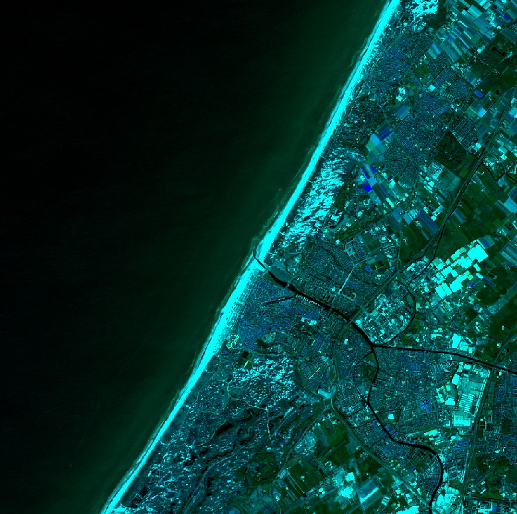
First, let’s assume that we have a GeoTiff image as follows:

Extract bounding box, SRID and number of bands

We can extract the bounding box, srid, and number of bands of this raster.

SELECT raster, RS_Envelope(raster) as bbox, RS_Metadata(raster), RS_NumBands(raster)
FROM rasterTable

+--------------------+--------------------+-----+--------+
|              raster|                geom| srid|numBands|
+--------------------+--------------------+-----+--------+
|GridCoverage2D["g...|POLYGON ((590520 ...|32631|       3|
+--------------------+--------------------+-----+--------+

Now this resulting table has a schema that contains both raster and geometry type (see below)

root
 |-- raster: raster (nullable = true)
 |-- geom: geometry (nullable = true)
 |-- srid: integer (nullable = true)
 |-- numBands: integer (nullable = true)

This allows for more complex geometric operations on the table. For instance, we can save the table as a GeoParquet format and perform filter pushdown. When executing a Sedona spatial range query on this GeoParquet table, Sedona will retrieve only the data that intersects the spatial range query window.

sedona.table("rasterTable").write.format("geoparquet").save("rasterTable.parquet")

Extract individual band

We can extract any band in a raster.

SELECT RS_BandAsArray(raster, 1) as band1, RS_BandAsArray(raster, 2) as band2,
 RS_BandAsArray(raster, 3) as band3
FROM rasterTable

+--------------------+--------------------+--------------------+
|               band1|               band2|               band3|
+--------------------+--------------------+--------------------+
|[0.0, 799.0, 788....|[0.0, 555.0, 546....|[0.0, 330.0, 322....|
+--------------------+--------------------+--------------------+

Modify a band value

We can modify a band value and save it to the original raster

SELECT RS_AddBandFromArray(raster, RS_GreaterThan(band1, 0), 1) AS raster)
FROM rasterTable

The resulting GeoTiff looks like this

Google S2-based spatial join (v1.4.0)

If you’re experiencing suboptimal performance with Sedona’s optimized join, it may be due to complicated and overlapping geometries. Fortunately, Sedona offers a built-in alternative: the Google S2-based approximate equi-join. This equi-join utilizes Spark’s internal equi-join algorithm and may perform better than the optimized join, especially if you choose to skip the refinement step. However, be aware that skipping the refinement step will result in a loss of query accuracy.

Sedona’s approximate equi-join is a useful tool to have in your arsenal when working with complex geometries. And with the recent updates to Sedona, such as the introduction of the native raster data type and the redesigned end-to-end raster ETL pipeline, Sedona is better equipped than ever to meet the evolving needs of the geospatial data processing community.

1. Generate S2 ids for both tables

Use ST_S2CellIds to generate cell IDs. Each geometry may produce one or more IDs.

SELECT id, geom, name, explode(ST_S2CellIDs(geom, 15)) as cellId
FROM lefts

SELECT id, geom, name, explode(ST_S2CellIDs(geom, 15)) as cellId
FROM rights

2. Perform equi-join

Join the two tables by their S2 cellId

SELECT lcs.id as lcs_id, lcs.geom as lcs_geom, lcs.name as lcs_name, rcs.id as rcs_id, rcs.geom as rcs_geom, rcs.name as rcs_name
FROM lcs JOIN rcs ON lcs.cellId = rcs.cellId

3. Optional: Refine the result

Due to the nature of S2 Cellid, the equi-join results might have a few false-positives depending on the S2 level you choose. A smaller level indicates bigger cells, less exploded rows, but more false positives.

To ensure the correctness, you can use one of the Spatial Predicates to filter out them. Use this query instead of the query in Step 2.

SELECT lcs.id as lcs_id, lcs.geom as lcs_geom, lcs.name as lcs_name, rcs.id as rcs_id, rcs.geom as rcs_geom, rcs.name as rcs_name
FROM lcs, rcs
WHERE lcs.cellId = rcs.cellId AND ST_Contains(lcs.geom, rcs.geom)

As you see, compared to the query in Step 2, we added one more filter, which is ST_Contains, to remove false positives. You can also use ST_Intersects and so on.

!!!tip
You can skip this step if you don’t need 100% accuracy and want faster query speed.

4. Optional: De-duplicate

Due to the explode function used when we generate S2 Cell Ids, the resulting DataFrame may have several duplicate <lcs_geom, rcs_geom> matches. You can remove them by performing a GroupBy query.

SELECT lcs_id, rcs_id , first(lcs_geom), first(lcs_name), first(rcs_geom), first(rcs_name)
FROM joinresult
GROUP BY (lcs_id, rcs_id)

The first function is to take the first value from a number of duplicate values.

If you don’t have a unique id for each geometry, you can also group by geometry itself. See below:

SELECT lcs_geom, rcs_geom, first(lcs_name), first(rcs_name)
FROM joinresult
GROUP BY (lcs_geom, rcs_geom)

Try it now

With these improvements and additions, Apache Sedona 1.4 s better equipped to meet the evolving needs of the geospatial data processing community.

We are immensely grateful to our fantastic community for their ongoing support and contributions to the development and growth of Apache Sedona. We are excited to continue our journey together, pushing the boundaries of geospatial data processing.

Stay tuned for future updates and enjoy your data processing with Apache Sedona 1.4!