Analyzing Real Estate Data With Apache Sedona
In a recent tutorial on the Wherobots YouTube channel we explored how to analyze real estate data using Apache Sedona and Wherobots Cloud using data from Zillow. Specifically, we calculated the change in median home value over the last 5 years per county using Zillow’s Zillow Home Value Index (ZHVI) and visualized the results. This […]
TABLE OF CONTENTS
In a recent tutorial on the Wherobots YouTube channel we explored how to analyze real estate data using Apache Sedona and Wherobots Cloud using data from Zillow. Specifically, we calculated the change in median home value over the last 5 years per county using Zillow’s Zillow Home Value Index (ZHVI) and visualized the results.
This tutorial highlights a few features of Apache Sedona and Wherobots Cloud, including:
- An overview of the Wherobots Cloud notebook environment
- How to upload data to Wherobots Cloud
- How to import datasets using Apache Sedona (CSV and Shapefile)
- Using SQL to query data using Apache Sedona
- Creating interactive visualizations of the results of our geospatial analysis in the Wherobots notebook environment
- Creating choropleth maps with GeoPandas and matplotlib
Feel free to follow along with the video tutorial below:
We used two data sources for this map:
- Zillow’s home values dataset (ZHVI) – CSV
- Natural Earth’s Admin 2 – Counties – Shapefile
To follow along create a free account in Wherobots Cloud and create a new blank notebook. We’ll be using Python and SQL to interact with Sedona.
Many geospatial Python packages are installed by default in Wherobots Cloud, but we can also add packages either when launching the notebook environment in the Wherobots Cloud UI or installing with pip in the notebook. For this tutorial the only package we’ll need to install is mapclassify which we’ll use to help with creating the data distribution bins when creating our choropleth map.
# All other packages are installed by default in Wherobots Cloud

pip install mapclassify
Next, we’ll import some dependencies for working with Sedona and importing our datasets.
from sedona.spark import *
from sedona.core.formatMapper.shapefileParser import ShapefileReader
from sedona.utils.adapter import Adapter
import geopandas
One of the first steps to using Sedona in our notebook is configuring the SedonaContext and connecting to our cluster. The config object here is typically where we can specify authentication providers for accessing cloud storage buckets. We won’t need this functionality in this tutorial, but this is the default configuration I typically use.
config = SedonaContext.builder().appName('zillowdata')\
    .config("spark.hadoop.fs.s3a.bucket.wherobots-examples-prod.aws.credentials.provider","org.apache.hadoop.fs.s3a.AnonymousAWSCredentialsProvider")\
    .getOrCreate()
sedona = SedonaContext.create(config)
Natural Earth Shapefile Import
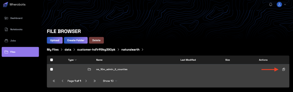
We’ll be analyzing real estate values at the county level in the US. Since the dataset from Zillow doesn’t include county geometries we’ll use the Natural Earth Admin Level 2 dataset for US county geometries. I uploaded the Shapefile files to Wherobots Cloud using this structure:
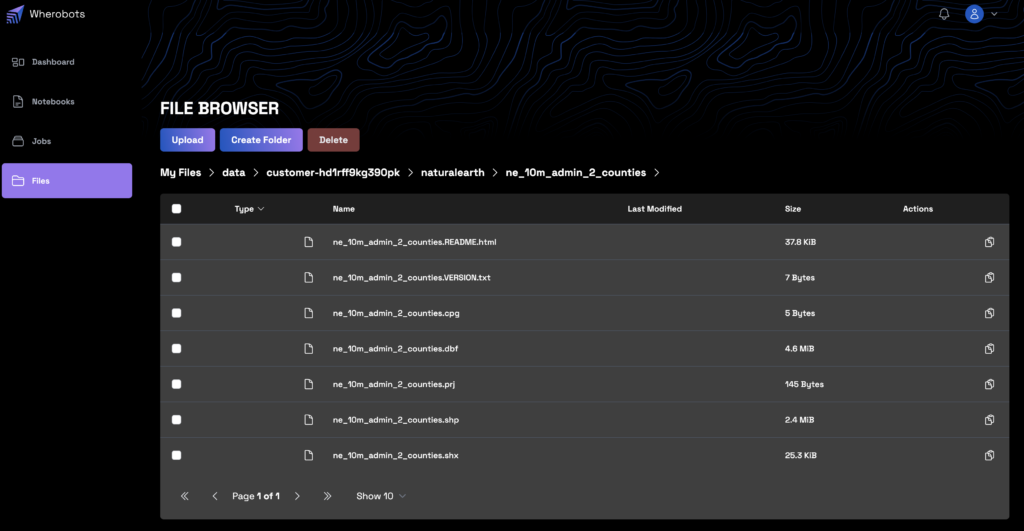
Note that since a Shapefile is composed of multiple files, the S3 URL we want to use is the location of the directory, not one of the individual files:
Then in our notebook we can save the S3 URL as a variable.
S3_URL_NE = "s3://<YOUR_S3_URL_HERE>"To import Shapefile datasets into Sedona we can use Sedona’s ShapefileReader to create a Spatial RDD data structure, then convert that Spatial RDD to a Spatial DataFrame, which we’ll then be able to query using Spatial SQL, after creating a view (or temporary table) from the DataFrame. Spatial RDDs are one of Sedona’s core data structures that extends the Spark RDD by enabling spatial geometries and querying functionality. Spatial DataFrames extend Spark DataFrames as well, offering spatial indexing, partitioning, and querying functionality.
spatialRDD = ShapefileReader.readToGeometryRDD(sedona, S3_URL_NE)
counties_df = Adapter.toDf(spatialRDD, sedona)
counties_df.createOrReplaceTempView("counties")
counties_df.printSchema()
We can inspect the schema of the county data we imported. The relevant columns for our use case are geometry (the polygon that represents the boundary of each county), FIPS (a unique identifier for each county), NAME_EN (the English name of the county), and REGION (the state).
root
 |-- geometry: geometry (nullable = true)
 |-- FEATURECLA: string (nullable = true)
 |-- SCALERANK: string (nullable = true)
 |-- ADM2_CODE: string (nullable = true)
 |-- ISO_3166_2: string (nullable = true)
 |-- ISO_A2: string (nullable = true)
 |-- ADM0_SR: string (nullable = true)
 |-- NAME: string (nullable = true)
 |-- NAME_ALT: string (nullable = true)
 |-- NAME_LOCAL: string (nullable = true)
 |-- TYPE: string (nullable = true)
 |-- TYPE_EN: string (nullable = true)
 |-- CODE_LOCAL: string (nullable = true)
 |-- REGION: string (nullable = true)
 |-- REGION_COD: string (nullable = true)
 |-- ABBREV: string (nullable = true)
 |-- AREA_SQKM: string (nullable = true)
 |-- SAMEASCITY: string (nullable = true)
 |-- LABELRANK: string (nullable = true)
 |-- NAME_LEN: string (nullable = true)
 |-- MAPCOLOR9: string (nullable = true)
 |-- MAPCOLOR13: string (nullable = true)
 |-- FIPS: string (nullable = true)
 |-- SOV_A3: string (nullable = true)
 |-- ADM0_A3: string (nullable = true)
 |-- ADM0_LABEL: string (nullable = true)
 |-- ADMIN: string (nullable = true)
 |-- GEONUNIT: string (nullable = true)
 |-- GU_A3: string (nullable = true)
 |-- MIN_LABEL: string (nullable = true)
 |-- MAX_LABEL: string (nullable = true)
 |-- MIN_ZOOM: string (nullable = true)
 |-- WIKIDATAID: string (nullable = true)
 |-- NE_ID: string (nullable = true)
 |-- latitude: string (nullable = true)
 |-- longitude: string (nullable = true)
 |-- NAME_AR: string (nullable = true)
 |-- NAME_BN: string (nullable = true)
 |-- NAME_DE: string (nullable = true)
 |-- NAME_EL: string (nullable = true)
 |-- NAME_EN: string (nullable = true)
 |-- NAME_ES: string (nullable = true)
 |-- NAME_FA: string (nullable = true)
 |-- NAME_FR: string (nullable = true)
 |-- NAME_HE: string (nullable = true)
 |-- NAME_HI: string (nullable = true)
 |-- NAME_HU: string (nullable = true)
 |-- NAME_ID: string (nullable = true)
 |-- NAME_IT: string (nullable = true)
 |-- NAME_JA: string (nullable = true)
 |-- NAME_KO: string (nullable = true)
 |-- NAME_NL: string (nullable = true)
 |-- NAME_PL: string (nullable = true)
 |-- NAME_PT: string (nullable = true)
 |-- NAME_RU: string (nullable = true)
 |-- NAME_SV: string (nullable = true)
 |-- NAME_TR: string (nullable = true)
 |-- NAME_UK: string (nullable = true)
 |-- NAME_UR: string (nullable = true)
 |-- NAME_VI: string (nullable = true)
 |-- NAME_ZH: string (nullable = true)
 |-- NAME_ZHT: string (nullable = true)
Now we can query this data using SQL:
sedona.sql("""
SELECT geometry, FIPS AS fips, NAME_EN AS name, REGION AS state FROM counties LIMIT 10
""").show()
+--------------------+-------+------------+-----+
| geometry| fips| name|state|
+--------------------+-------+------------+-----+
|MULTIPOLYGON (((-...|US53073| Whatcom| WA|
|POLYGON ((-120.85...|US53047| Okanogan| WA|
|POLYGON ((-118.83...|US53019| Ferry| WA|
|POLYGON ((-118.21...|US53065| Stevens| WA|
|POLYGON ((-117.42...|US53051|Pend Oreille| WA|
|POLYGON ((-117.03...|US16021| Boundary| ID|
|POLYGON ((-116.04...|US30053| Lincoln| MT|
|POLYGON ((-114.72...|US30029| Flathead| MT|
|POLYGON ((-114.06...|US30035| Glacier| MT|
|POLYGON ((-112.19...|US30101| Toole| MT|
+--------------------+-------+------------+-----+Load Zillow ZHVI CSV File
Now that we have the geometries of each county we want to import the CSV file with the Zillow home value index data. I uploaded this file into Wherobots Cloud as well which we can access in our notebook environment using the S3 URL copied from the file browser UI.
S3_URL_ZHVI = "s3://<YOUR S3 URL HERE>"After importing the CSV file into a new DataFrame we create a view and print the schema to inspect the data.
zhvi_df = sedona.read.format('csv').option('header','true').option('delimiter', ',').load(S3_URL_ZHVI)
zhvi_df.createOrReplaceTempView("zhvi")
zhvi_df.printSchema()
root
|-- RegionID: string (nullable = true)
|-- SizeRank: string (nullable = true)
|-- RegionName: string (nullable = true)
|-- RegionType: string (nullable = true)
|-- StateName: string (nullable = true)
|-- State: string (nullable = true)
|-- Metro: string (nullable = true)
|-- StateCodeFIPS: string (nullable = true)
|-- MunicipalCodeFIPS: string (nullable = true)
|-- 2000-01-31: string (nullable = true)
|-- 2000-02-29: string (nullable = true)
|-- 2000-03-31: string (nullable = true)
...
|-- 2023-10-31: string (nullable = true)So our Zillow data has information about the county and a column for each monthly home value index going back to the year 2000 (I’ve omitted several column names from the output above).
Let’s inspect the first few rows of our Zillow data:
sedona.sql("""
SELECT RegionName,StateName, State, Metro, StateCodeFIPS, MunicipalCodeFIPS, `2000-01-31` FROM zhvi LIMIT 10
""").show()
+------------------+---------+-----+----------+-------------+-----------------+-------------+
| RegionName|StateName|State| Metro|StateCodeFIPS|MunicipalCodeFIPS| 2000-01-31|
+------------------+---------+-----+----------+-------------+-----------------+-------------+
|Los Angeles County| CA| CA|Los Ang...| 06| 037| 205974.69363|
| Cook County| IL| IL|Chicago...| 17| 031| 145499.51956|
| Harris County| TX| TX|Houston...| 48| 201|108350.203359|
| Maricopa County| AZ| AZ|Phoenix...| 04| 013|143352.154097|
| San Diego County| CA| CA|San Die...| 06| 073| 214883.41007|
| Orange County| CA| CA|Los Ang...| 06| 059|249870.608658|
| Kings County| NY| NY|New Yor...| 36| 047|200000.033597|
| Miami-Dade County| FL| FL|Miami-F...| 12| 086| 119546.52618|
| Dallas County| TX| TX|Dallas-...| 48| 113| 94256.230613|
| Riverside County| CA| CA|Riversi...| 06| 065| 149474.98732|
+------------------+---------+-----+----------+-------------+-----------------+-------------+Joining ZHVI And County Geometries
So we now have two tables zhvi and counties – let’s join them together so we can plot current home value per county. To do that we’ll use the FIPS code which uniquely identifies each county. The zhvi table breaks the FIPS code out into the state and municipal components so we’ll need to combine them so we can join against the counties table.
zhvi_county_df = sedona.sql("""
SELECT CAST(zhvi.`2023-10-31` AS float) AS value, zhvi.RegionName As name, counties.geometry
FROM zhvi
JOIN counties
ON CONCAT('US', zhvi.StateCodeFIPS, zhvi.MunicipalCodeFIPS) = counties.FIPS
WHERE NOT zhvi.State IN ('HI', 'AK')

zhvi_county_df.show(5)
""")
+---------+-------------------+--------------------+
| value| name| geometry|
+---------+-------------------+--------------------+
|582171.56| Whatcom County|MULTIPOLYGON (((-...|
|300434.03| Okanogan County|POLYGON ((-120.85...|
| 279648.9| Ferry County|POLYGON ((-118.83...|
|365007.16| Stevens County|POLYGON ((-118.21...|
|364851.38|Pend Oreille County|POLYGON ((-117.42...|
+---------+-------------------+--------------------+
only showing top 5 rowsNow that we have our home value index and the county geometry in a single DataFrame we can use a choropleth map to visualize the data geographically. The SedonaPyDeck package supports creating choropleths with the create_choropleth_map method.
SedonaPyDeck.create_choropleth_map(zhvi_county_df,plot_col="value")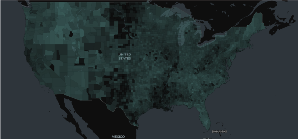
We can also use matplotlib to create a choropleth by converting our zhvi_county_df Sedona DataFrame to a GeoDataFrame. A best practice when creating choropleth maps is to use an equal area projection to minimize distortion of the areas being visualized so we set the CRS of our GeoDataFrame to Albers Equal Area.
zhvi_gdf = geopandas.GeoDataFrame(zhvi_county_df.toPandas(), geometry="geometry")
zhvi_gdf.to_crs(epsg=3857)
Now we can plot our data as a choropleth using matplotlib. We’ll specify a yellow-green color ramp and experiment with different binning schemes that best fit the distribution of the data we’re visualizing. Here we use the Jenks-Caspall method.
ax = zhvi_gdf.plot(
    column="value",
    scheme="JenksCaspall",
    cmap="YlGn",
    legend=True,
    legend_kwds={"title": "Median Home Value($)", "fmt": "{:.0f}", "loc": "lower right"},
    missing_kwds={
        "color": "lightgrey",
        "edgecolor": "red",
        "hatch": "///",
        "label": "Missing values"
    },
    figsize=(12,9)
)

ax.set_axis_off()
ax.set_title("Median Home Value By County, Oct 2023")
ax.annotate("Data from Zillow, 2023 ZHVI",(-125,25))

plt.savefig("zhvi.png",dpi=300)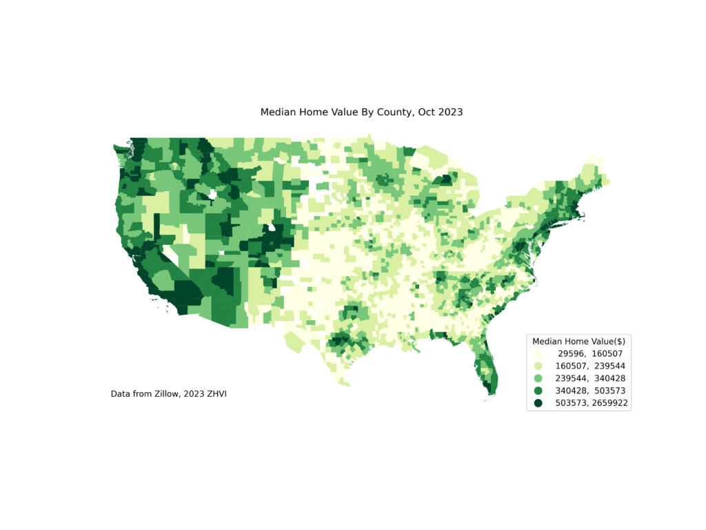
Visualizing Change In Home Value
So far we’ve plotted the current home value, now let’s calculate the change in home value over the last 5 years and visualize the spatial distribution.
In our SQL query let’s calculate the percent change in home value from 2018 to 2023. We’ll also compute the centroid of each county so we can annotate the map.
delta_county_df = sedona.sql("""
SELECT
  ((CAST(zhvi.`2023-10-31` AS float) - CAST(zhvi.`2018-10-31` AS float)) / (CAST(zhvi.`2018-10-31` AS float)) * 100 )  AS delta,
  zhvi.RegionName As name, zhvi.Statename AS state,counties.geometry, ST_Centroid(counties.geometry) AS centroid
FROM zhvi
JOIN counties
ON CONCAT('US', zhvi.StateCodeFIPS, zhvi.MunicipalCodeFIPS) = counties.FIPS
WHERE NOT zhvi.State IN ('HI', 'AK')
""")delta_county_df.show(5)+-----------------+-------------------+-----+--------------------+--------------------+
| delta| name|state| geometry| centroid|
+-----------------+-------------------+-----+--------------------+--------------------+
|52.68140223225829| Whatcom County| WA|MULTIPOLYGON (((-...|POINT (-121.71238...|
|55.31723313387478| Okanogan County| WA|POLYGON ((-120.85...|POINT (-119.73730...|
|32.94520356645385| Ferry County| WA|POLYGON ((-118.83...|POINT (-118.51643...|
|66.86739887826734| Stevens County| WA|POLYGON ((-118.21...|POINT (-117.85278...|
|66.78068227229824|Pend Oreille County| WA|POLYGON ((-117.42...|POINT (-117.27525...|
+-----------------+-------------------+-----+--------------------+--------------------+We follow similar steps as above to create a GeoDataFrame.
# We'll convert to a GeoDataFrame

delta_gdf = geopandas.GeoDataFrame(delta_county_df.toPandas(), geometry="geometry")
delta_gdf.to_crs(epsg=3857)
Let’s find the counties with the most extreme changes in home value so we can annotate them on the map.
To find the county with the greatest increase in property value:
delta_gdf.iloc[delta_gdf['delta'].idxmax()]delta 169.532379
name Petersburg City
state VA
geometry POLYGON ((-77.40366881899992 37.23746578695217...
centroid POINT (-77.39189306391864 37.20426989798888)
Name: 2937, dtype: objectAnd to find the county with the greatest decrease in property value:
delta_gdf.iloc[delta_gdf['delta'].idxmin()]delta -44.794506
name Claiborne Parish
state LA
geometry POLYGON ((-93.23859537841794 33.01169686180804...
centroid POINT (-92.99522452214245 32.81998668151367)
Name: 944, dtype: objectThe steps to create our choropleth map using matplotlib are similar to the previous map however this time since our data diverges around zero we’ll use a red-yellow-green color ramp and manually specify the bins.
ax = delta_gdf.plot(
    column="delta",
    scheme="User_Defined",
    cmap="RdYlGn",
    legend=True,
    legend_kwds={"title": "Median Home Value % Change", "loc": "lower right"},
    classification_kwds={"bins":[0,20,40,60,80,100,170]},
    missing_kwds={
        "color": "lightgrey",
        #"edgecolor": "red",
        #"hatch": "///",
        "label": "Missing values"
    },
    figsize=(12,9)
)

ax.set_axis_off()
ax.set_title("Median Home Value Percent Change By County, 2018-2023")
ax.annotate("Data from Zillow's ZHVI",(-125,25))

ax.annotate('Petersburg City, VA +169.5%',
            xy=(-77.39189306391864, 37.20426989798888), xycoords='data',
            xytext=(100, 10), textcoords='offset points',
            arrowprops=dict(facecolor='black', shrink=0.05),
            horizontalalignment='center', verticalalignment='bottom')

ax.annotate('Claiborne Parish, LA -44.8%',
            xy=(-92.99522452214245, 32.81998668151367), xycoords='data',
            xytext=(50, -110), textcoords='offset points',
            arrowprops=dict(facecolor='black', shrink=0.05),
            horizontalalignment='center', verticalalignment='bottom')

plt.savefig("delta.png", dpi=300)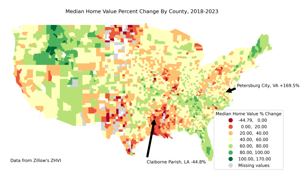
Even though we didn’t leverage much advanced Spatial SQL functionality this post demonstrated how to work with spatial data in various formats (CSV and Shapefile) in Wherobots Cloud, how to use SQL with Apache Sedona to join datasets, and how to leverage tools from the PyData ecosystem like GeoPandas and matplotlib in the Wherobots Notebook environment.
Resources
In addition to the data sources linked at the beginning of this post, I found the following resources helpful when creating this map:
- Choropleth Mapping chapter from Geographic Data Science With Python book
- GeoPandas mapping and plotting tools documentation
- Matplotlib example of annotating plots
- StackOverlow answer on using manual breakpoints for matplotlib classes
Create your free Wherobots Cloud account today to get started working with geospatial data and Apache Sedona
Want to keep up with the latest developer news from the Wherobots and Apache Sedona community? Sign up for the This Month In Wherobots Newsletter: